
From Theory to Evidence: Translating Hypotheses into Regression Specifications#
Regression is a useful tool for exploring research questions. In the previous section we reviewed several uses of regression analysis in practice — extrapolation, causal inference, predictive modeling. In this section we focus on a step that precedes all of them: how one gets from a theory, or a research question, to a concrete regression specification. We start with an example that we develop step by step, and close by showing that the same process repeats, with the same pieces, across business research more broadly.
1. From Theory to Hypothesis#
One common way of thinking about the quantitative research process is the following sequence:
A theory is a coherent set of ideas or claims intended to explain a phenomenon or behavior. A theory in marketing, for example, might propose that trust generates loyalty. A proposition is exactly that: a specific statement that connects concepts that, in principle, we could observe. A hypothesis goes one step further: it proposes a relationship between measurable variables that, given a dataset, can actually be tested. The rest of this section walks through these three steps with a concrete example, and ends by showing how the hypothesis, in turn, becomes a regression equation.
2. An Example: Customer Trust and Loyalty#
The theory#
Take a subscription platform — think of something like Netflix or Airbnb — that wants to understand what drives customer loyalty. The theory, in its simplest form, holds that better service quality builds customer trust, and that trust, in turn, builds loyalty.
“Service Quality,” “Trust,” and “Loyalty” are constructs: theoretical concepts that don’t exist as columns in any database. Beyond this chain, it’s reasonable to think there are factors that affect loyalty without going through trust: the customer’s tenure (months since they signed up) and the plan they’re on (for example, Basic or Premium). We call these controls.
The diagram#
Before writing down any equation, it helps to represent this theory as a diagram: constructs and arrows, still no variables.
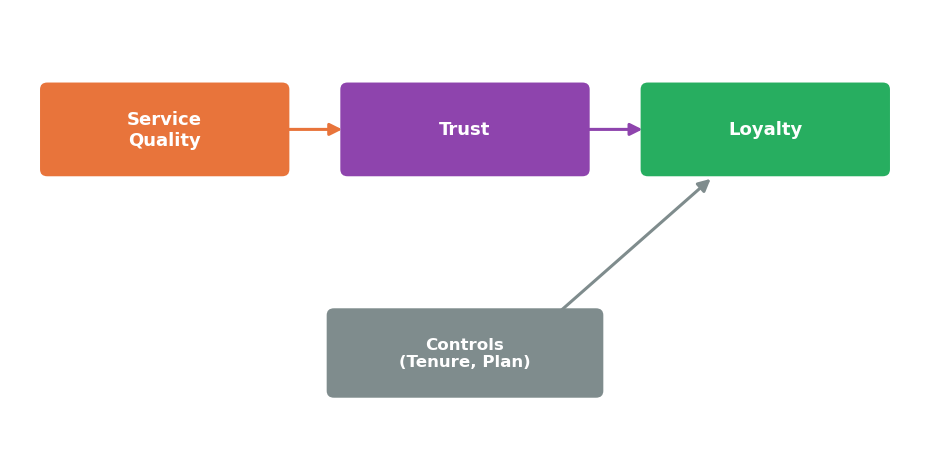
Each arrow in the diagram is a relationship the theory proposes. None of them is yet expressed in terms of measurable variables — that’s the next step.
The propositions#
The diagram above implies two concrete propositions:
P1: service quality increases customer trust.
P2: customer trust increases loyalty.
From propositions to hypotheses#
None of the three constructs is directly observable. To test them, we need to assume we can measure them with concrete variables — their proxies. Suppose we measure Service Quality with technical-support response time and the platform’s uptime percentage; we measure Trust with the average satisfaction rating a customer reports after each support interaction (on a 1-to-5 scale); and we measure Loyalty with a renewal indicator for the customer’s quarter.
With these variables, the propositions above become testable hypotheses:
H1: a shorter response time and a higher uptime are associated with a higher satisfaction rating.
H2: a higher satisfaction rating is associated with a higher probability of renewal.
It’s worth noting that no proxy is perfect — the rating a customer leaves after one interaction is not their trust in the company, it’s a number subject to every kind of noise (how their day was going, how recently an issue was resolved). This distinction between construct and proxy is the one most often lost when someone jumps straight from a theory to a regression without passing through this intermediate step.
3. From Data to Equation#
As we saw with the Google/Meta/Amazon compensation model in the previous section, any hypothesis expressed in measurable variables can be thought of, in its most general form, as a still-unknown mathematical function connecting those variables. Let’s take H2 to see how this idea translates into an equation — the same procedure would apply to H1.
H2 suggests there’s a function \(f\) connecting the customer’s satisfaction rating, tenure, and plan to their probability of renewing:
We still don’t know what shape \(f\) takes — only that, if H2 is correct, this function exists. Writing a regression model we can actually work with amounts, at bottom, to choosing a concrete form for \(f\). The simplest one, and this book’s starting point, is to assume \(f\) is linear — as we’ll see in the next section, this isn’t the only option, but it’s the most direct place to start:
where \(i\) indexes the customer, and \(\varepsilon_i\) absorbs everything else that affects renewal and isn’t on the right-hand side: other omitted determinants, and also the noise that comes from using an imperfect proxy in place of the true construct.
Note: the unit of analysis
Before fixing this equation, there’s a decision that often gets made without noticing: what counts as “one observation”? Above, the natural answer is the customer — each row of the dataset is a customer, with their own satisfaction rating and their own renewal history. But that’s not the only option. We could instead define the observation as a customer-quarter (if we want to capture how loyalty changes over time), or even the market (if we’re asking, say, whether markets with higher average brand trust retain more customers overall). Each choice of unit of analysis implies a different dataset and, often, a slightly different research question. Fixing it — deliberately, not by default — is part of translating theory into a concrete research design. In our example the unit of analysis is the customer: each observation \(i\) is a single customer.
This equation — and the question of how to estimate it, how to interpret \(\beta_1\), and under what conditions that number reflects anything like a causal relationship — is exactly what the rest of the book teaches you to answer. We’ll start by asking what, formally, is the best possible version of a function like \(f\) — the conditional expectation function — and then, in Regression Mechanics I and II, revisit the decision we made above to assume \(f\) is linear, first with one explanatory variable and then with several.
4. The Pattern Repeats Across the Business#
The process we just walked through — theory, diagram, propositions, hypotheses, equation — is, in essence, the subject matter of business research. It shows up, with the same pieces, in practically any area of a business that uses data to make decisions. Pick an area to see a concrete case: in each one you’ll be able to spot the constructs, their proxies, and the implicit unit of analysis, just as we did above.
Marketing: Price Elasticity of Demand
Objective: price elasticity of demand is one of the most common regressions in applied marketing: it estimates how much quantity sold moves in response to a price change, controlling for promotion and advertising. The log-log specification gives \(\beta_1\) a direct interpretation as an elasticity — key input for pricing and promotion planning.
Reference: Hanssens, Parsons, and Schultz (2001), Market Response Models.
Finance: CAPM and Expected Return
Objective: the CAPM (Capital Asset Pricing Model) is central to financial theory: it proposes that an asset's expected excess return has a linear relationship with the expected excess return of the market portfolio, where \(\beta_i\) measures the asset's exposure to market-wide risk. It underlies performance evaluation and investment decisions.
Reference: Sharpe (1964); extended into a multi-factor model by Fama and French (1993).
HR: The Gender Pay Gap
Objective: the Oaxaca-Blinder decomposition splits an observed gap — here, the gender pay gap — into a portion explained by differences in observable characteristics (education, experience) and an unexplained residual, often attributed to discrimination. It remains one of the standard tools compensation-analytics teams use to audit pay equity.
Reference: Oaxaca (1973).
Operations: Wait Time and Satisfaction
Objective: measures how support wait time affects customer satisfaction, net of whether the issue was actually resolved — the kind of model a SaaS support team runs to decide whether to invest in faster response times or better first-contact resolution.
Reference: no specific citation in the original source for this example.
Strategy: Determinants of Firm Performance
Objective: Rumelt's variance-decomposition approach asks how much of the spread in firm profitability is attributable to the industry a firm competes in versus firm-specific factors — informing whether a firm's strategy should focus on picking the right industry or building unique capabilities within it.
Reference: Rumelt (1991).
Full references for these five models appear in the References section at the end of this page: [Hanssens et al., 2001], [Sharpe, 1964], [Fama and French, 1993], [Oaxaca, 1973], [Rumelt, 1991].
With this walkthrough — from theory to diagram, from diagram to proposition, from proposition to hypothesis, and from hypothesis to equation — you’re now equipped to recognize a regression specification the next time you see one, in this book or anywhere else. The next step is to start seeing exactly how that equation gets estimated.
References#
Eugene F Fama and Kenneth R French. Common risk factors in the returns on stocks and bonds. Journal of Financial Economics, 33(1):3–56, 1993.
Dominique M Hanssens, Leonard J Parsons, and Randall L Schultz. Market Response Models: Econometric and Time Series Analysis. Kluwer Academic Publishers, 2001.
Ronald Oaxaca. Male-female wage differentials in urban labor markets. International Economic Review, 14(3):693–709, 1973.
Richard P Rumelt. How much does industry matter? Strategic Management Journal, 12(3):167–185, 1991.
William F Sharpe. Capital asset prices: a theory of market equilibrium under conditions of risk. Journal of Finance, 19(3):425–442, 1964.