Instrumental Variables: Two-Stage Least Squares and Weak Instruments#
In the previous section we derived the LATE estimator as the ratio of the reduced form and first stage, using a binary instrument. That logic generalizes naturally to situations where the instrument and the treatment are continuous, and where there may be additional control variables. The standard method for implementing this generalization is two-stage least squares (2SLS).
This section presents the estimation procedure, explains why incorrect handling of standard errors produces wrong inference, introduces the use of multiple instruments, and analyzes the problem of weak instruments — instruments with a first stage too small to identify the causal effect precisely.
1. Objectives#
By the end of this section, you will be able to:
Implement the 2SLS estimator in two steps and understand why the first-stage fitted values are “clean.”
Identify why manual 2SLS standard errors are incorrect and how to fix them.
Incorporate multiple instruments into the first stage and evaluate the precision gain.
Describe the two harms caused by a weak instrument: bias toward OLS and over-rejection of the null.
Interpret the first-stage F-statistic as a continuous measure of instrument strength, without anchoring to discrete thresholds.
2. From Binary Logic to the General Case: 2SLS#
The previous section used a binary instrument \(Z \in \{0, 1\}\) and derived the LATE as a difference of conditional means. In practice, instruments and treatments are often continuous, and models include control variables. 2SLS generalizes the Wald estimator to this setting.
The new Uber example: The platform wants to estimate how hours worked on the platform (\(T\) = weekly active hours) affect driver weekly earnings (\(Y\)). The unobservable confounder \(U\) is driver motivation: more motivated drivers work more hours and earn more per hour (better routes, higher trip acceptance rates), so a regression of earnings on hours overstates the causal effect of hours.
The instrument is notification intensity (\(Z_1\) = number of push notifications sent by the platform to the driver during the week). More notifications nudge drivers to log on — first stage: \(Z_1 \rightarrow T\). The number of notifications is determined by the platform algorithm based on aggregate trip demand, not on individual driver quality — exogeneity: \(Z_1 \perp U\). The notification contains no information about hourly rates or driving strategies — exclusion restriction: \(Z_1 \not\rightarrow Y\) directly.
The IV DAG for the continuous case has the same structure as the binary case:
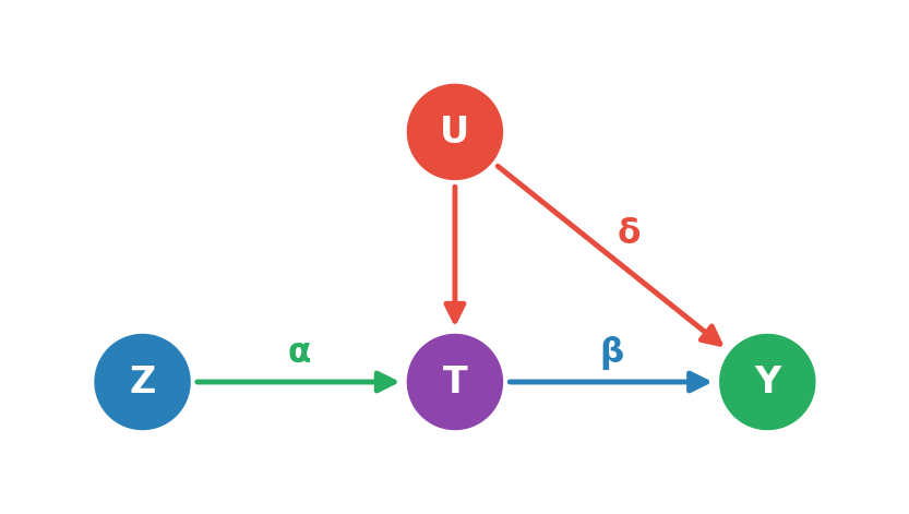
Legend: \(Z_1\) — Notification intensity · \(T\) — Hours on platform · \(Y\) — Weekly earnings · \(U\) — Driver motivation (unobs.)
2.1 How the 2SLS estimator works#
The 2SLS is an estimation method that allows recovering the LATE using two consecutive OLS regressions. It is defined as follows:
First stage: Regress the treatment \(T\) on the instrument \(Z_1\) (and any control variables \(X\)):
Save the fitted values:
Second stage: Regress the outcome \(Y\) on the fitted values \(\hat{T}\) (and the same controls \(X\)):
The coefficient \(\hat{\beta}\) from the second stage is the 2SLS estimate of the causal effect.
2.2 Why \(\hat{T}\) is “clean”#
The logic of the method is the same as in the binary case: the fitted values \(\hat{T}_i\) capture only the variation in \(T\) that comes from the instrument \(Z_1\) — the exogenous component. The endogenous component — the part of \(T\) correlated with \(U\) — lives in the first-stage residual \(\hat{e}_i = T_i - \hat{T}_i\), which is excluded from the second stage.
By regressing \(Y\) on \(\hat{T}\) rather than on \(T\), the second stage can no longer capture the effect of \(U\) on \(Y\) through its correlation with \(T\): that channel was eliminated when \(T\) was projected onto the instruments.
2.3 Connection to the LATE estimator#
When \(Z_1\) is binary and there are no additional controls, the 2SLS estimator reduces exactly to the Wald ratio:
In the continuous case with controls, the second-stage coefficient retains the interpretation of a local causal effect — the variation it identifies is exactly what the instrument generates in \(T\).
3. The Problem with Manual Standard Errors#
Running the two stages manually — as two consecutive OLS regressions — gives the correct point estimate but incorrect standard errors.
The problem lies in the second-stage residuals. If the second stage is estimated as OLS on \(\hat{T}\), the residuals are:
But \(\hat{T}_i\) is “smoother” than \(T_i\): it excludes the first-stage noise (\(\hat{e}_i\)). This causes the residuals \(\hat{v}_i\) to over-absorb variance, inflating the manual standard error estimate relative to the correct value. In this type of DGP (confounding-based endogeneity), the manual 2SLS standard error is too wide, not too narrow.
The correct formula uses residuals computed against the original treatment \(T_i\), not \(\hat{T}_i\):
This adjustment — and other corrections related to the two-stage structure — is implemented automatically by specialized software packages (linearmodels.IV2SLS in Python, ivreg in R). Never report standard errors from a manually constructed 2SLS.
4. Multiple Instruments#
When more than one valid instrument is available, all can be included in the first stage to extract more exogenous variation from \(T\). Consider the following example.
A second instrument for Uber: In addition to notification intensity (\(Z_1\)), the platform ran a parallel campaign randomly mailing branded driver gear to a subset of drivers (\(Z_2 = 1\) if the driver received the package — items such as a phone mount, car freshener, and co-branded accessories). Receiving the gear package increases motivation to use the platform, nudging drivers to log on more hours — first stage: \(Z_2 \rightarrow T\). The mailing list was generated independently of individual driver quality — exogeneity: \(Z_2 \perp U\). The gear items themselves do not change per-hour earnings or the structure of fares — their only route to affecting earnings is through the additional hours driven on the platform — exclusion restriction, plausible under this design.
The first stage with two instruments:
More valid instruments mean more exogenous variation in \(T\) available for the second stage, translating into a higher first-stage F-statistic and a narrower confidence interval on \(\beta\).
5. Consolidation via Simulation: Scenario A#
With the 2SLS mechanism formalized, the simulation lets you walk through both stages visually and observe the concrete consequence of the standard error problem.
Before exploring, predict:
In LATE view, what relationship should you see between the reduced-form slope, the first-stage slope, and the LATE ratio?
In 2SLS view, which variation in \(T\) appears on the x-axis of the second-stage plot?
Why does the manual 2SLS standard error appear in amber? Is it wider or narrower than the correct one?
When you increase \(\gamma_1\) from 0.2 to 1.5, what happens to the first-stage F and the confidence interval on \(\beta\)?
The left panel shows the first-stage scatter (\(T\) on \(Z_1\)); the estimated slope is \(\hat{\gamma}_1\). In 2SLS view, the overlay of gold diamond markers shows the \(\hat{T}_i\) values — exactly the points passed to the second stage. The right chart then shows the second stage (\(Y\) on \(\hat{T}\)), whose slope is \(\hat{\beta}\).
The coefficient table at the bottom compares OLS, manual 2SLS (standard error in amber — incorrect, too wide), and software 2SLS (correct). The point estimate is identical in the latter two; only the standard errors differ. In LATE view, the computation table shows numerically that LATE = \(\hat{\gamma}_{RF}/\hat{\gamma}_{FS}\) equals the 2SLS coefficient.
6. Weak Instruments#
A weak instrument is one whose first stage is small relative to the sampling noise. The consequence is not a specification error but a continuous degradation of the 2SLS estimator’s properties.
6.1 The two harms of a weak instrument#
1. Bias toward OLS in finite samples. When \(\gamma_1\) is small, \(Z_1\) barely moves \(T\). The exogenous variation the instrument extracts is tiny; the second stage becomes dominated by estimation noise. In the limit (\(\gamma_1 \rightarrow 0\)), 2SLS converges to the OLS estimator: if the instrument says nothing about \(T\), the estimation is equivalent to regressing \(Y\) directly on \(T\), with all the selection bias that implies.
2. Over-rejection of the null. The asymptotic approximations that justify standard 2SLS inference assume the instrument has a first-order effect on \(T\). When that effect is weak, the approximations deteriorate: confidence intervals undercover the true parameter and hypothesis tests reject too often.
6.2 Instrument strength is continuous, not binary#
Instrument weakness is not a discrete condition. As the first-stage F-statistic approaches 1, IV bias converges monotonically toward OLS bias and standard confidence intervals undercover increasingly. There is no single threshold that separates a “good” instrument from a “bad” one. The relevant question is not “does F exceed some value?” but “how much additional bias am I willing to accept, and at what cost in variance?”
The most cited convention — proposed by Staiger and Stock [1997] — reports the first-stage F as an indicator and notes that values around 10 guarantee that IV bias is less than 10% of OLS bias under certain conditions. That reference point is worth knowing, but it has an obvious limitation: it is expressed relative to OLS bias, not in absolute terms. If OLS bias is small, a modest F may be sufficient; if OLS bias is large, even an F well above 10 may leave appreciable IV bias. Treating F = 10 as a binary cutoff between “good” and “bad” obscures this gradualness.
6.3 Practical guidance#
Always report the first-stage F (and first-stage \(R^2\)) so readers can evaluate instrument strength.
A strong instrument that violates the exclusion restriction remains inconsistent. Strength does not compensate for invalidity.
7. Consolidation via Simulation: Scenario B#
With the notion of instrument weakness clear, the second scenario of the simulation lets you directly observe the continuous degradation of the IV estimator as the instrument weakens, and the benefit of having a second valid instrument.
Before exploring, predict:
What happens to the sampling distribution of the IV estimator when you lower \(\gamma_1\) from 1.50 to 0.05?
Does IV bias shift discretely (a “break”) or continuously?
When you enable two instruments and set both to \(\gamma_1 = \gamma_2 = 0.40\), how does the joint F change relative to one instrument with \(\gamma_1 = 0.40\)?
What is the difference between reducing IV bias by using a stronger single instrument versus using two moderate instruments?
The F-gauge at the top of the right panel changes color continuously — from red (F near 1) through amber to teal (F large) — with no discrete zones or marked thresholds. That visual continuity is intentional: it reflects that estimator degradation is gradual, not a jump at some cutoff. The density curves below show the sampling distributions of OLS (red) and IV (blue) across 500 Monte Carlo realizations: as \(\gamma_1\) decreases, the blue curve widens and its center shifts continuously toward OLS bias. Enabling the second instrument (\(Z_2\)) raises the joint F and narrows the blue curve — more exogenous variation available, better estimation.
The statistics table at the bottom summarizes the mean, standard deviation, and coverage rate of both estimators for the current parameters.
Test what you learned#
References#
The interactive dashboard in this section also draws on Angrist and Pischke [2009], Stock and Watson [2020], and Andrews et al. [2019], in addition to Staiger and Stock [1997].
Isaiah Andrews, James H Stock, and Liyang Sun. Weak instruments in instrumental variables regression: theory and practice. Annual Review of Economics, 11:727–753, 2019.
Joshua D Angrist and Jörn-Steffen Pischke. Mostly harmless econometrics: An empiricist's companion. Princeton university press, 2009.
Douglas Staiger and James H Stock. Instrumental variables regression with weak instruments. Econometrica, 65(3):557–586, 1997.
James H Stock and Mark W Watson. Introduction to Econometrics. Pearson, 4th edition, 2020.