The Conditional Expectation Function: From Averages to a Model

The Conditional Expectation Function: From Averages to a Model#

Ask an HR analyst what a technical-track employee with 8 years of experience typically earns, and they’ll give you a number — an average. That number is already a model, whether anyone calls it one or not. It’s useful for predicting what a new employee with that profile would earn, but it could also serve as a basis for explaining the salary differences associated with experience: why does someone with more years in the role earn more? What exactly is that number, formally, and how well does it serve each of those two roles?

This section answers that question. We’ll start from a very simple idea — averaging \(Y\) for each value of \(X\) — and we’ll see, by playing with data, what this idea’s strengths and limits are: what non-linear relationships and what systematic differences between groups it’s capable of revealing, and why estimating it well is not as simple as defining it. Out of that will come the central object of this section, the Conditional Expectation Function (CEF), and a first, concrete reason why the rest of the book is devoted to estimating it with a regression model rather than averaging group by group.

1. Objectives#

By the end of this section you’ll be able to:

Define the Conditional Expectation Function, \(m(x) = E[Y \mid X=x]\), and recognize its estimation as the natural generalization of “average by group” to any variable \(X\).
Estimate it empirically — by averaging \(Y\) among observations that share a value of \(X\) — and explain why that estimate gets noisy when few observations share the same value.
Explain why a regression model can approximate the CEF with less data than averaging value by value, and what’s gained and lost by doing so.
Place next section’s equation, \(Y = \beta_0 + \beta_1 X + \varepsilon\), as a special — linear — case of this more general idea.

2. A first look at the data#

Throughout this section we’ll work with one running example: a technology company, and a sample of its employees with two figures per person — annual salary (in thousands of USD) and years of experience — plus a third variable, career track: Technical or Managerial.

Here’s what 200 employees of this company look like, with no fitting or summarizing at all:

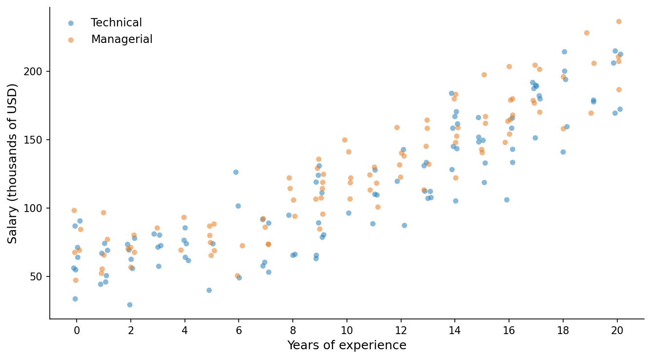
Scatter of salary against years of experience, by track

The cloud is genuinely noisy. Even so, something is visible at a glance: the orange points (Managerial) look systematically higher than the blue ones (Technical), and within each color salary seems to rise with experience, though not in a perfectly tidy way. The question guiding the rest of this section is: what’s the best way to summarize this cloud with one number per experience level, rather than a single number for everyone?

3. Estimating an average, one experience value at a time#

Experience here is measured in whole years — so the most direct answer is: for each experience value, average the salary of every employee with exactly that many years. Try it yourself.

In the dashboard below you’ll control the sample size and two overlays. Before reading the interpretation in the next subsection, notice:

With small samples (n=50), how consistent are the empirical CEF points from one experience value to the next? Are there values where the point strays far from its neighbors?
The count bar below the chart — are the most erratic CEF points sitting above tall bars or short ones?
Turn “Split by track” on and off — what happens to the pooled CEF relative to the two separate CEFs?
At n=5000, do the points look tidier than at n=50? What changed — the data, or the estimator?

4. Naming what you just built: the CEF#

What you just built by hand in the dashboard — group by value of \(X\), then average \(Y\) within each group — is an estimate of the object this section is named for, the Conditional Expectation Function (CEF):

\[m(x) = E[Y \mid X=x]\]

It’s worth being precise here, because the two are easy to conflate. The CEF, \(m(x)\), is a population object: the expected value of \(Y\) in the subpopulation where \(X=x\), a fixed property of the joint distribution of \((X,Y)\) that doesn’t depend on any particular sample. What you did in the dashboard — grouping your sample’s observations by value of \(X\) and averaging \(Y\) within each group — is how that object is estimated, not the object itself. And it’s precisely estimating it that way that is the natural generalization of “average by group” to any variable \(X\), not just a category: if \(X\) were a categorical variable (say, track), estimating \(m(x)\) would simply mean averaging \(Y\) within each category of the sample — something you probably already knew how to do. When \(X\) is a number, like experience, the same idea applies: group by every possible value and average.

That estimator — the sample average at each value of \(X\) — is unbiased for \(m(x)\); the proof is in the appendix at the end of the section.

This connects directly to something left open earlier: up to now we’ve characterized the relationship between \(X\) and \(Y\) through an unknown function \(F\), of the form \(Y = F(X) + \varepsilon\). Under fairly general conditions, the \(F\) that best describes the relationship is the CEF: \(F(x) = m(x) = E[Y \mid X=x]\). It is, in a precise sense, the best possible answer to “what value of \(Y\) do I expect, given that I know \(X\)?”.

5. Why estimating the CEF is, fundamentally, a data problem#

The dashboard above showed something worth formalizing: as the number of cells (distinct values of \(X\)) grows relative to the sample size, each cell receives fewer observations, and the average within that cell becomes more variable. With few observations, an average can end up dominated by two or three employees with unusual salaries — pure sampling bad luck, not a flaw in the model.

This is not a failure of the CEF as a concept: the population CEF, \(m(x)\), is a fixed, well-defined object, and its estimator — the sample average at each value of \(X\) — is unbiased (see the proof in the appendix). The problem is one of precision, not bias: the more cells there are to fill with the same amount of data, the more thinly the sample is stretched, and the noisier each individual estimate becomes. It’s a genuine trade-off between granularity (how many distinct values of \(X\) you distinguish) and precision (how reliable the average is at each one) — not a defect that more data, or a different strategy, can’t address.

6. A more efficient way to approximate the CEF#

The dashboard above leaves an open problem: averaging by each experience value splits the sample into smaller and smaller compartments as the number of distinct \(X\) values grows — you gain resolution, but lose precision. Is there a way to get both?

Here’s the intuition: instead of estimating an independent average for each value of \(X\), a parametric model — say, a line, or a line with a kink — imposes a specific functional form on \(m(x)\), and that form is estimated using the entire sample at once, not a fraction of it per value of \(X\). The model “borrows strength” from neighboring observations instead of treating each value of \(X\) as an isolated problem. That’s, in essence, the bet a regression model makes — and it’s what you’ll compare, head to head with the empirical CEF, in the next dashboard.

7. Comparing the empirical CEF to regression, head to head#

Choose a model in the left-hand panel and see how well it fits the same sample. Before reading the interpretation:

At n=50, compare the RMSD (root mean squared distance to the true population CEF) of “Regression + track dummy and kink” against “CEF by bins.” Which is lower?
Now move to n=5000 and see what happens to the RMSD of “Pooled regression” (which ignores track and the kink). Did it improve much?
Compare that same transition (n=50 → n=5000) for “CEF by bins” and for “Regression + track dummy and kink.” Which of the two improved more with added data?
What do the models that don’t improve much with more data have in common?

8. Regression as a parametric CEF#

What you saw in the dashboard can be formalized like this: a regression model is nothing more than a way of imposing a specific functional form on \(m(x)\), in exchange for needing far less information at any individual point.

When that functional form is correct — in the dashboard, a line with a kink at the promotion threshold plus a constant level difference between tracks — the fitted model gets closer to the true CEF than the empirical CEF does, even with small samples: it doesn’t split the data into compartments, it uses all of it together to estimate a handful of parameters. When the functional form is wrong — like the pooled regression, which ignores track and the kink — the model is biased: systematically wrong in certain regions, an error that no amount of additional data corrects, unlike the empirical CEF’s noise, which does shrink with more sample.

This trade-off — committing to a functional form in exchange for efficiency — is, in one sentence, what the rest of the book’s regression chapters are about: a model like the one that won in the dashboard, with a slope that changes at one point and a constant shift between groups, is something you’ll learn to build precisely starting in the next section.

9. Closing: what’s next, and one honest simplification#

With this, we can pick back up the notation left open earlier: we had been writing the relationship between \(X\) and \(Y\) as \(Y = F(X) + \varepsilon\), without saying much about \(F\). We now know that the best candidate for \(F\), in the sense of lowest mean squared error, is the CEF: \(F(x) = m(x) = E[Y \mid X=x]\). The next section takes the natural next step: assuming that \(F\) has a linear form, and showing how it’s estimated.

One clarification before moving on. This section’s example used two explanatory variables — experience and track — to show both a non-linearity (the kink) and a systematic difference between groups. Regression Mechanics I deliberately steps back and works with a single explanatory variable, to build the mechanics of regression as clearly as possible. It’s not a step backward: Regression Mechanics II brings back multiple explanatory variables — including categorical variables like track — now with the tools needed to handle them properly.

Appendix: Formal proofs#

A.1 The conditional sample average is an unbiased estimator of the CEF#

Fix a particular value \(x\), and let \(n_x\) be the number of sample observations with \(X_i = x\). The estimator you used in the dashboard is:

\[\hat m(x) = \frac{1}{n_x}\sum_{i \,:\, X_i = x} Y_i\]

Each \(Y_i\) among those \(n_x\) observations is, by construction, a draw from the distribution of \(Y\) conditional on \(X=x\) — so, by the definition of the CEF, \(E[Y_i \mid X_i = x] = m(x)\) for each one of them. Taking the conditional expectation given that cell’s composition:

\[E\big[\hat m(x) \mid X_i = x \text{ for the } n_x \text{ observations in the cell}\big] = \frac{1}{n_x}\sum_{i \,:\, X_i = x} E[Y_i \mid X_i = x] = \frac{1}{n_x}\sum_{i \,:\, X_i = x} m(x) = m(x)\]

The sample average at each value of \(X\) is, then, exactly unbiased for \(m(x)\) — not “in principle,” but as a direct consequence of the CEF’s definition. What varies with \(n_x\) is not the bias, but the precision: the variance of \(\hat m(x)\) is \(\text{Var}(Y \mid X=x)/n_x\), which shrinks with \(\sqrt{n_x}\), just like the variance of any sample average.

A.2 The CEF’s error has zero conditional mean#

Define \(\varepsilon = Y - m(X)\). Conditional on \(X=x\), \(m(X)\) is a constant (equal to \(m(x)\)), so:

\[E[\varepsilon \mid X=x] = E[Y - m(X) \mid X=x] = E[Y \mid X=x] - m(x) = m(x) - m(x) = 0\]

The last equality uses the CEF’s own definition, \(E[Y \mid X=x] = m(x)\). The result holds for every \(x\), so \(E[\varepsilon \mid X] = 0\).

A.3 The CEF minimizes the mean squared prediction error#

For any function \(g(X)\), add and subtract \(m(X)\) inside the squared prediction error:

\[E[(Y-g(X))^2] = E\big[\big((Y-m(X)) + (m(X)-g(X))\big)^2\big] = E[(Y-m(X))^2] + 2\,E[(Y-m(X))(m(X)-g(X))] + E[(m(X)-g(X))^2]\]

The cross term vanishes by the law of iterated expectations and result A.2:

\[E[(Y-m(X))(m(X)-g(X))] = E\Big[\big(m(X)-g(X)\big)\,\underbrace{E[Y-m(X)\mid X]}_{=\,0 \text{ by A.2}}\Big] = 0\]

So:

\[E[(Y-g(X))^2] = E[(Y-m(X))^2] + E[(m(X)-g(X))^2] \;\ge\; E[(Y-m(X))^2]\]

since the second term is a square and can’t be negative. Equality holds only when \(g(X) = m(X)\) (with probability 1) — that is, \(g=m\) is the unique function that minimizes the mean squared error. No other function of \(X\), linear or not, can predict \(Y\) better, in this sense, than the CEF.